Table of Contents
- Introduction
- Fundamental Decibel Equation
- Power to dB Conversion Table
- Example Calculations
- Voltage to Power Conversion
- Time Domain Representation
Introduction
Decibels (dB) are a logarithmic unit used to express the ratio of a quantity to a reference value, enabling a more manageable representation of magnitudes spanning large ranges. Decibels are one-tenth of a Bel, a unit named after Alexander Graham Bell. The most common application of decibels is in expressing power ratios, although they can also be applied to other quantities such as voltage.
Fundamental Decibel Equation
The fundamental formula for calculating the power ratio in Bels is:
\[\Large log_{10}\left(\frac{P}{P_{ref}}\right) = P_{Bel}\]However, decibels (dB) are more commonly used in practice. To convert from Bels to decibels, the value is multiplied by 10:
\[\Large 10 \cdot log_{10} \left (\frac{P}{P_{ref}} \right) = P_{dB}\]Where:
- \(\Large P\) is the power value to be converted.
- \(\Large P_{ref}\) is the reference power level in the same units as P.
Power to dB Conversion Table
The table below provides a reference for converting specific power levels to decibels relative to one mW (dBm).
| Power Level | dBm |
|---|---|
| 1000 W | 60 |
| 100 W | 50 |
| 10 W | 40 |
| 1 W | 30 |
| 100 mW | 20 |
| 10 mW | 10 |
| 1 mW | 0 |
| 100 uW | -10 |
| 10 uW | -20 |
| 1 uW | -30 |
| 100 nW | -40 |
| 10 nW | -50 |
| 1 nW | -60 |
Example Calculations
To illustrate the application of the decibel formula, consider the following example calculations for power levels in watts, converted to dBm. It is essential to note that both the input power and the reference power should be expressed in the same units. For consistency and to minimize errors, using base units such as watts is recommended.
5 Watts
Given a power level of 5 Watts, the decibel value relative to 1 milliwatt (dBm) is calculated as follows:
\[\Large 10 \cdot \log_{10} \left( \frac{5}{100e-3} \right) = 36.9897 \text{ dBm}\]1 Watt
Given a power level of 1 Watts, the decibel value relative to 1 milliwatt (dBm) is calculated as follows:
\[\Large 10 \cdot \log_{10} \left( \frac{1}{100e-3} \right) = 30.0 \text{ dBm}\]Voltage to Power Conversion
In certain applications, such as radio frequency (RF) systems, it may be necessary to convert voltage to power. This requires knowledge of the system’s impedance. It is important to note that this calculation assumes a purely sinusoidal waveform with no DC offset and a purely resistive impedance. Although this method provides a close approximation, it is not intended to yield analytically precise values.
The process begins with the basic decibel equation, but the power ($P$) term is calculated using Ohm’s law derivation. Note that there are many alternative forms of the combined equation that are mathematically equivalent.
Ohm’s Law Derivation
Starting with Ohm’s law which states \(P = V \cdot I\) and recognizing that current (\(I\)) can be expressed as \(\Large \frac{V}{R}\), we substitute into the power equation:
\[\Large P = \frac{V}{R} \cdot V = \frac{V^2}{R}\]This formula provides the power as a function of the system resistance $R$ and applied voltage, $V$.
RMS Voltage Calculation
For AC signals, such as those in RF applications, the RMS voltage should be used unless instantaneous power is to be calculated. For a signal such as a sine wave the RMS value represents the average voltage of the signal. In other words the DC equivalent. The RMS factor will change depending on the signal waveform.
In the case of a pure sine wave the voltage is calculated by dividing the peak voltage by \(\sqrt{2}\).
\[\Large V_{rms} = \frac{V_{pk}}{\sqrt{2}} \approx \frac{V_{pk}}{1.414}\]Recall that the peak voltage for a pure sine wave is half the peak to peak voltage.
Complete Equation for Power Calculation
Combining the derived expressions yields the final equation for calculating power, in dBm, from the peak voltage of a sine wave within a system of known impedance.
\[\Large 10 \cdot log_{10}\left(\frac{\left(\frac{V_{pk}}{\sqrt{2}}\right)^2}{P_{ref} \cdot Z_0}\right) = P_{dBm}\]Where:
- \(\Large V_{pk}\) is the peak sine wave voltage, in volts.
- \(\Large P_{ref}\) is the reference power level. 1mW (1e-3 W) in the case of dBm.
- \(\Large Z_0\) is system impedance, typically $50 \Omega$ in most RF systems.
- \(\Large P_{dBm}\) is the calculated output power, in units of dBm.
Power from Voltage Example
Provided the previous equation, calculate the power, in dBm, of a \(5V_{pk}\) sine wave in a \(50 \Omega\) system.
\[\Large 10 \cdot log_{10}\left(\frac{\left(\frac{5}{\sqrt{2}}\right)^2}{0.001 \cdot 50}\right) = 23.9794_{dBm}\]Time Domain Representation
Calculations provided illustrate operating under steady state average conditions. When applying this function to a set of discrete instantaneous points within the time domain the results are not as intuitive. To illustrate the results the function is plotted below:
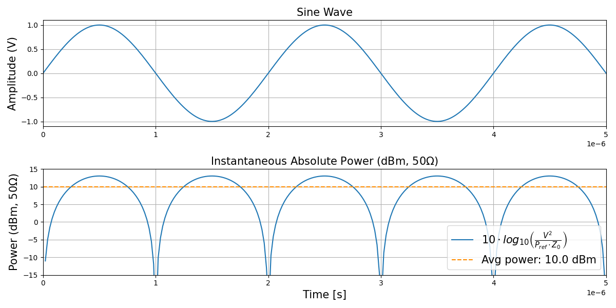
Note that the equation uses the absolute power and not the RMS equivalent. Using the average would allow using a max() function to find the average power at the peaks of the function. This method would be useful when using instruments such as an oscilloscope to avoid needing to post process data to obtain a result.
Code Snippet
#########################################
# Time domain voltage to decibel plot
# Author: LambdaFox
# Date: 24 August 2024
# Website: https://lambdafox.com
#
# Revision Log:
# 1.0.0 - Initial Release

import numpy as np
import matplotlib.pyplot as plt
from matplotlib.gridspec import GridSpec

# Waveform parameters
frequency       = 1e6 / 2
total_cycles    = 5
sampling_rate   = 100 * frequency
amplitude       = 1
time_period     = 1 / frequency
time            = np.linspace(0, total_cycles * time_period, int(sampling_rate * total_cycles * time_period))

# Generate the sine wave
sinewave = amplitude * np.sin(2 * np.pi * frequency * time)

# Calculate the power conversion function
rms_power = 10 * np.log10( ((sinewave) / np.sqrt(2)) ** 2 / (0.001 * 50) )
function_output = 10 * np.log10( ((sinewave ** 2) / (0.001 * 50) ))

# Create the figure and gridspec
fig = plt.figure(figsize=(12, 6))
gs = GridSpec(2, 1) # Two rows, one column

# Top Plot - Sine Wave
ax1 = fig.add_subplot(gs[0, 0])
ax1.plot(time, sinewave)
ax1.set_ylabel('Amplitude (V)', fontsize = 15)
ax1.set_title('Sine Wave', fontsize = 15)
ax1.set_xlim(0, 5e-6)
ax1.grid(True)

# Bottom Plot - Instantenous Absolute Power Plot
ax2 = fig.add_subplot(gs[1, 0])
ax2.plot(time, function_output, label = r'$10 \cdot log_{10}\left(\frac{V^2}{P_{ref} \cdot Z_0}\right)$')
ax2.axhline(np.nanmax(rms_power), linestyle='--', color= 'darkorange', label = f'Avg power: {np.nanmax(rms_power).round(3)} dBm')
ax2.set_ylabel('Power (dBm, $50 \Omega$)', fontsize = 15)
ax2.set_xlabel('Time [s]', fontsize = 15)
ax2.set_title('Instantaneous Absolute Power (dBm, 50$\Omega$)', fontsize = 15)
ax2.set_xlim(0, 5e-6)
ax2.set_ylim(-15, 15)
ax2.grid(True)
ax2.legend(fontsize = 15, loc='lower right')

plt.tight_layout()
plt.show()